
Muon lifetime measurement
I've heard about muons for the first time during my last year at school, when preparing for the physics exam at my university (NaUKMA in Kyiv, Ukraine). The teacher mentioned back then that there are these elementary particles coming from space that constantly pass through our bodies, without us ever noticing. It felt like science fiction.
Later, during the 3rd year into my BSc degree (Bachelor of Science), I've been studying history of Cosmic Ray discovery, as part of my assignment in scientific public speaking. And then later, during my PhD and post-doc, I've analysed real experimental data that was attributed to Cosmic Muons. While it felt closer than the old scientific articles, it was still just passive data to me that I had no control over.
My first actually interactive experience with Cosmic Muons was back in 2018, when I was offered to be a laboratory assistant at UniTO (University of Turin, Italy), building a muon-detection and data-acquisition system for students. This time I had the whole experimental apparatus in my hands, which made me feel like I can actually see those muons that are invisible to everyone else. And that's a pretty cool feeling.
Now, in 2026, when I had to come up with a laboratory experiment for my students, choosing Cosmic Muon detection has been a no-brainer. The only caveat is that it requires a lot of specialised equipment, which is not something that every university lab has. Luckily, at UPO (Università Piemonte Orientale) we have plenty, thanks to its involvement in several nuclear-physics experiments.
What I love about this experiment is that it combines several different disciplines:
- low-level programming and boolean logics;
- signal routing and time synchronisation;
- encoding and decoding of binary data;
- data visualisation;
- statistical analysis and modeling.
And even a small mistake at any point will ruin the outcome of the whole measurement, which trains the patience, discipline and attention to every detail.
Muons – what are they?
Muons are unstable elementary particles that are primarily produced in the upper atmosphere. When high energy protons and heavy ions arrive from the outer space, they collide with the nuclei of the atoms in the air molecules. Those collisions create pions, which almost immediately decay into muons and neutrinos. The muons are also unstable, but not as much. Their lifetime is long enough to reach the Earth surface before they decay, which is why we can detect them in the lab.
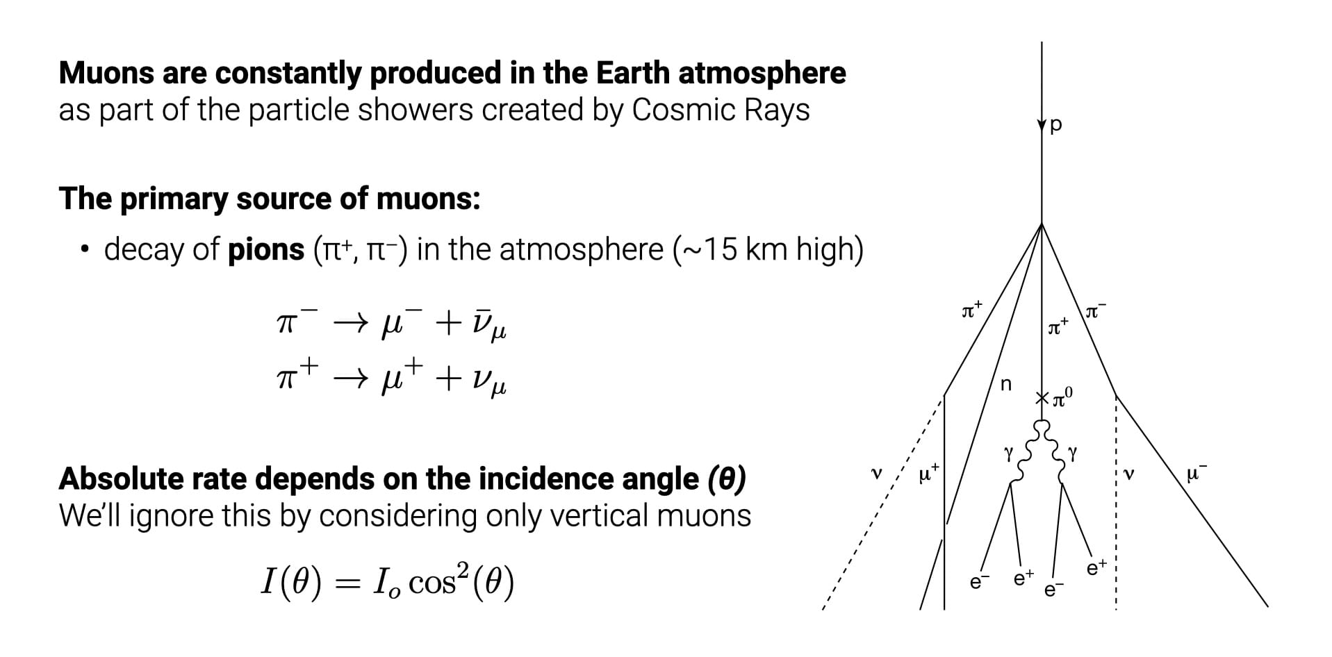
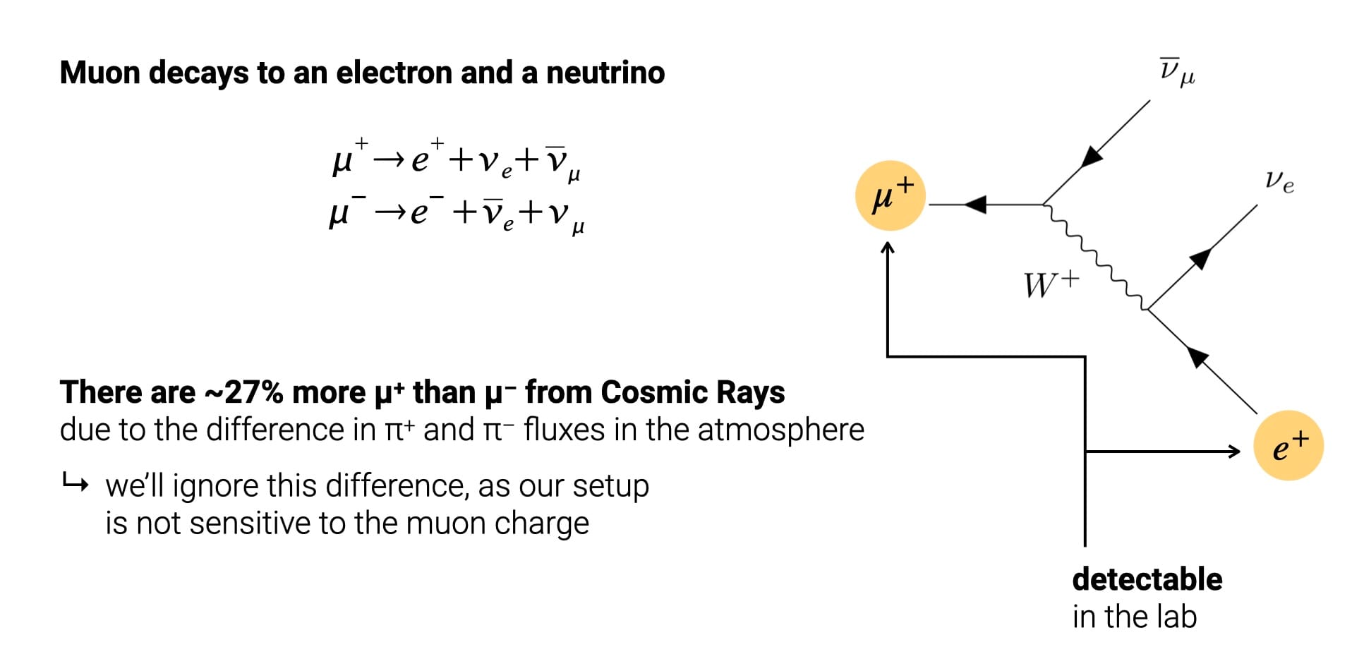
Muons are essentially like electrons, but about ⨉200 times heavier. They interact with matter very little, which allows them to pass sometimes through hundreds of metres of rock before they lose all their energy and stop. When they decay, two neutrinos and an electron are produced. Neutrinos almost never interact with matter, which makes them practically impossible to detect in the lab. Electrons, on the other hand, interact with matter much more and therefore we can detect them.
Mean lifetime – what is it?
Being elementary particles, muons follow the rules of quantum physics, where nothing is definite and everything is probabilistic. Therefore, when we say that a muon is unstable, it's impossible to tell when exactly it will decay. We can only talk about the probability of it decaying within a specific time window, and that is something that can be described mathematically and observed statistically.
When we observe a large number of muons, each decaying at its own unpredictable time, the collective quantity of them will follow the exponential-decay law, which is defined by the characteristic parameter 𝜏 (tau).
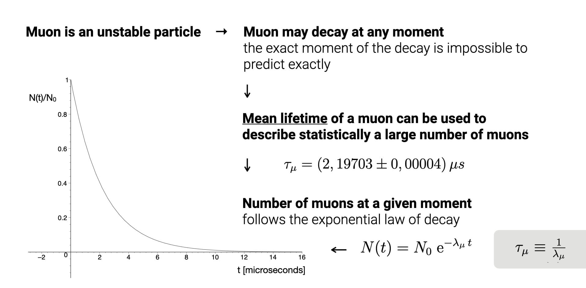
This parameter is what we call mean lifetime – the time in which the number of muons decreases by e (Euler's number = 2.718). This relation makes it easy to deduce this parameter from experimental data by simply measuring the amount of muons over time. If measured accurately, we should obtain a distribution that follows exactly the exponential curve with 𝜏 = 2.2 μs (microseconds), which is one of the fundamental constants of nature.
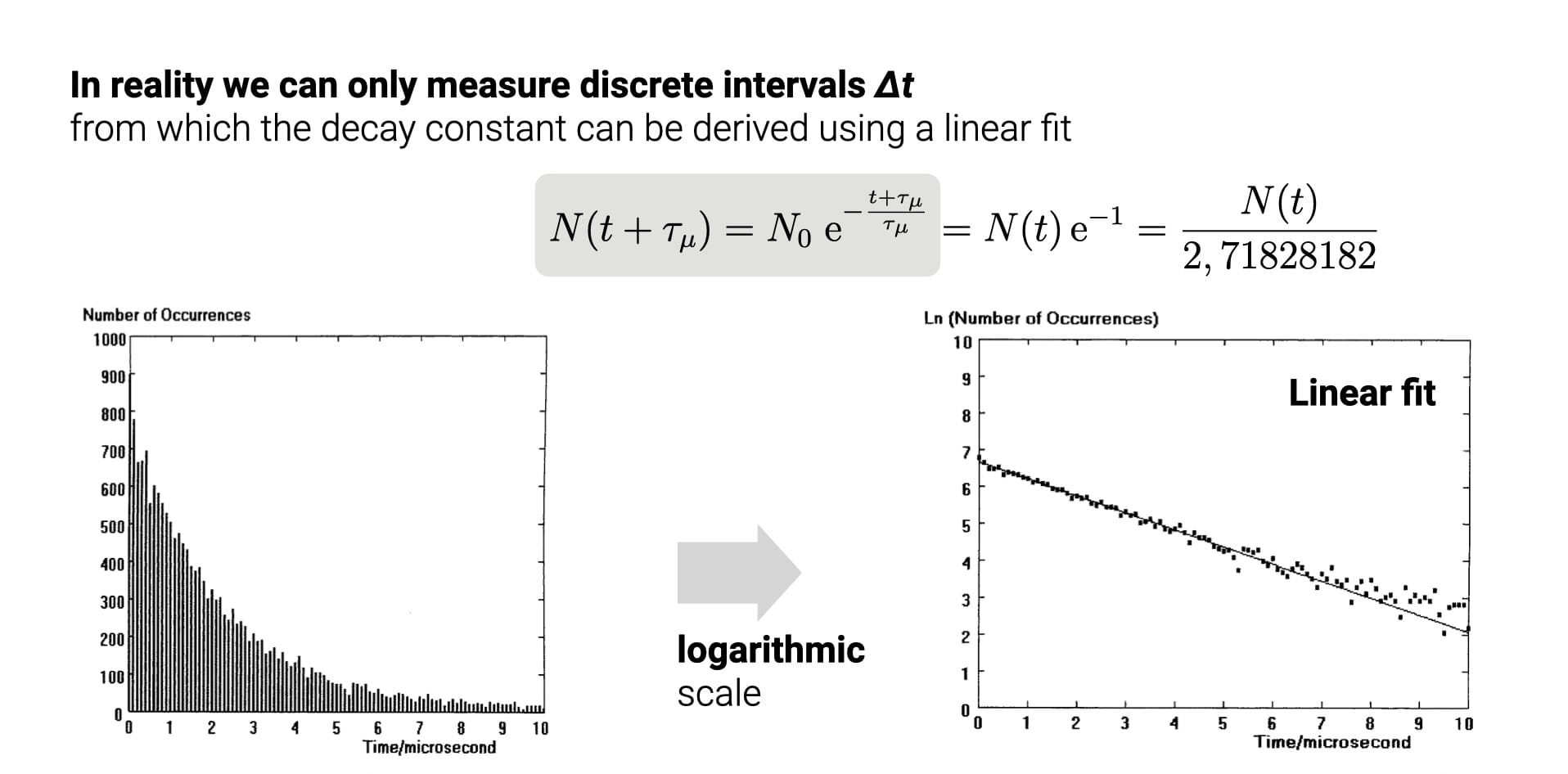
Measuring the number of muons at each time interval is equivalent to measuring the time between the muon's creation and the moment of its decay. It should follow an exponential curve with the same value of the parameter 𝜏.
Muon decay – how to measure it?
A typical way of measuring the muon decay is by using a scintillating material, which converts the energy lost in it by the particle into photons that can be registered by photosensors. In this particular case we use a big dense BGO (Bi4Ge3O12) crystal that has a higher chance of stopping muons within its volume, thanks to its high stopping power. Every muon entering the crystal will produce scintillation photons along its path, creating an instant flash of light.
When the muon stops, it loses its relativistic properties, so the time will start flowing for it at the same speed as for us in the lab, forcing it to decay within a few microseconds. When it decays, an electron is produced, which immediately starts losing its own energy in the crystal, creating a second flash of light.
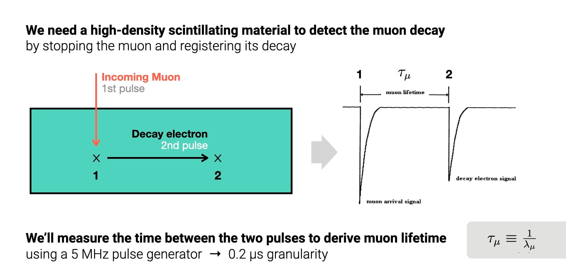
We register the scintillation photons with a PMT (photomultiplier tube) that is extremely sensitive, creating measurable pulses of current from single photons of light. Therefore, we can easily identify a muon decay when we observe two pulses in the PMT separated by a few microseconds. If we measure the time between these two pulses for a large number of muons, its distribution should follow that exponent that I've mentioned earlier.
An important caveat of such sensitive photo-sensors is that pulses of comparable amplitude can be created randomly by the thermal noise or by other energetic particles naturally present in the environment, for example beta particles or gamma rays. To suppress such random signals we add two more scintillators and a dense absorber in between, which only muons could pass through. If we require all the three scintillators to have pulses at exactly the same time, we can be confident that they were caused by a single muon passing vertically through all of them.
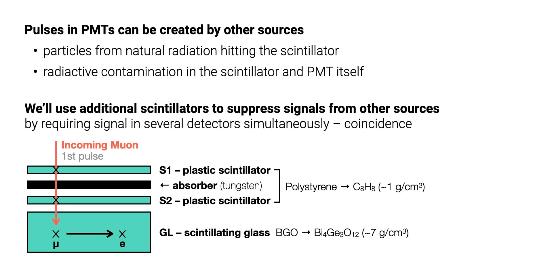
In this case we use blocks of tungsten as an absorber and plastic scintillators (C8H8) for the coincidence requirement. Since their purpose is to detect the passage of muons rather than to stop them, lightweight plastic is a better choice.
Data acquisition setup
Conceptually the goal of our experiment can be described with the following 3 steps:
- detect 3 simultaneous pulses in the three PMTs coupled to the scintillators
↳ START the timer; - detect a second pulse in the BGO crystal
↳ STOP the timer; - read the elapsed time and store it to a file.
If we run this for several days or weeks, we can collect enough measurements to get a smooth exponential distribution, from which the mean-lifetime parameter can be extracted though a least-square fit.
Implementing this in practice requires a lot of components with different functions that constitute the so-called DAQ (data acquisition) system. Based on the equipment available in our lab we have built it using two separate systems:
- NIM (National Instrumentation Methods) – supports various functions arranged in separate modules, such as threshold units, AND/OR functions, timers, pulse generators, multiplexers, etc.
- CAMAC (Computer Automated Measurement and Control) – supports programmable modules that can be controlled from a computer.
In this specific experiment only 2 CAMAC modules are necessary:
- Scaler to count input pulses from a pulse generator, which are then converted to elapsed time;
- I/O Register to detect and send changing logic levels in various NIM modules.
The following types of NIM modules are used in this experiment:
- discriminator (CAEN 96) to generate a logic TRUE signal when the input PMT pulse crosses a predefined threshold;
- coincidence unit (CAEN N455, LeCroy 465) to operate as AND/OR gate with one or more input logic signals;
- FAN-IN/FAN-OUT (LeCroy 428F) to distribute multiple copies of one input signal;
- pulse generator (custom by Silvano Gallian for INFN) to continuously generate square-wave pulses at 20 MHz frequency;
- delay (Phillips Scientific 792) to delay an input signal by up to 63.5 ns for precise time alignment of several signals;
- timer (CAEN N93B) to generate logic signals of various duration, representing distinctive states of the DAQ system.
Manual trigger
Given the large number of components, it's useful to first built the logic part of the DAQ without the actual detectors, so that the coincidence of 3 scintillators is generated by hand. This configuration uses 4 timer modules (TIMn), which have the following operating principle.
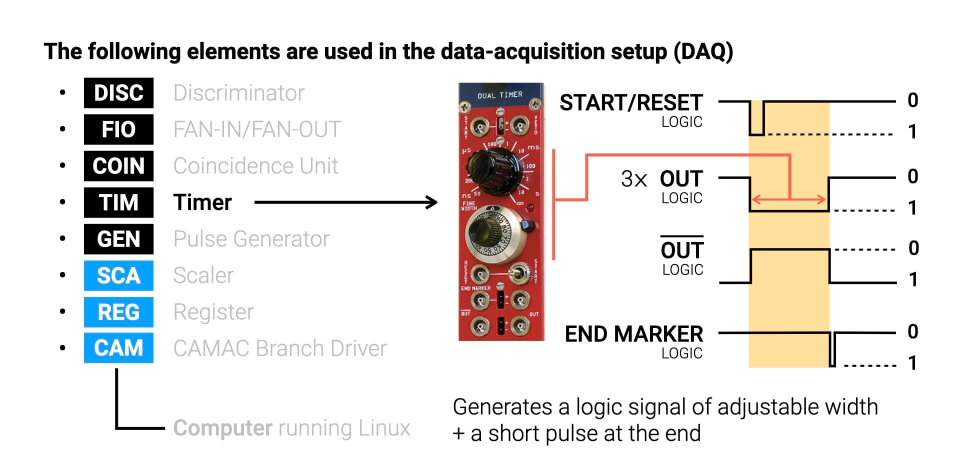
When a pulse arrives to the START input, it generates a pulse in its three OUT channels with the precise duration defined by the two knobs. It can range from nanoseconds to tens of seconds, or it can be set to Infinity, in which case OUT channels stay TRUE forever. At the end of the output pulse another short pulse is generated in the END MARKER channel as a sign that the timer has reached its configured duration. If at any moment the RESET input receives a pulse, all OUT channels return to FALSE. It also has a VETO input, used to ignore any START and RESET signals while the VETO level is TRUE. Finally, it has a little two-way switch that allows to generate a START or RESET signal by hand.
The scheme below shows the DAQ setup with a manual trigger activated by the START switch of the TIM4 module. Its time is set to a few microseconds, so that its OUT pulse mimics the 1st pulse from the BGO, while the END MARKER pulse mimics the 2nd pulse from the BGO.
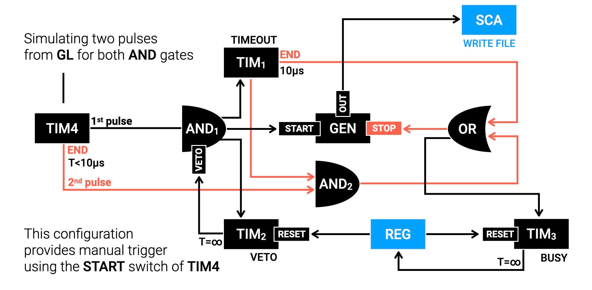
The main elements in this DAQ configuration are the following:
- AND1 represents the moment of coincidence from which we start counting the time, and wait for the 2nd BGO pulse;
- TIM2 sends an infinite VETO signal to AND1 to prevent it from generating any new triggers until we are finished with the current one;
- TIM1 defines the 10 µs timeout – the maximum time during which we are waiting for the 2nd BGO pulse;
- AND2 will generate a pulse only when the 2nd BGO pulse arrives, which has to happen while the TIM1 is still active;
- OR module sends a STOP signal to the pulse generator when either the 2nd BGO pulse has arrived or TIM1 has reached its timeout;
- TIM3 starts an infinite pulse representing the BUSY signal for the CAMAC+PC, during which the computer program has to detect the new trigger through the REG module, read the number of counted pulses from the SCA (Scaler) module and set RESET signals through the REG (Register) module, which then removes the VETO from AND1;
- at this point AND1 is ready to receive a new trigger to start the whole chain over again.
This cycle through steps 1-7 is executed every time we press the START switch of the TIM4 module. A dedicated C program must be running on the PC to actually read the Scaler, write the number of pulses to a data file, and then send the relevant RESET signals through the I/O Register.
Actual trigger with PMTs
Now we replace TIM4 with actual PMTs, whose signals pass through discriminators (DISC) – to select sufficiently large pulses, and delay units (DEL) – to correct for time differences due to the different response times of the scintillators and PMTs, different cable lengths and even the physical time of flight between scintillators.
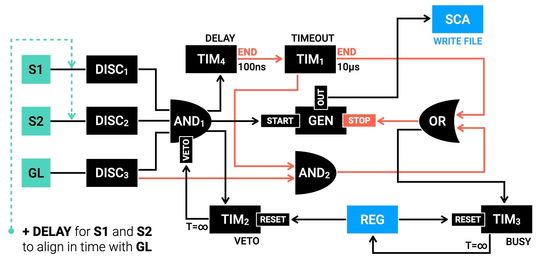
You can notice that we've added one more timer before TIM1 to create an additional delay after the START signal. This is necessary because the BGO pulse is quite slow, and it can take more than 100 ns for the PMT output to return to its baseline. During that time even very small pulses caused by thermal noise can add up and exceed the DISC3 threshold, leading to a fake STOP signal that wasn't caused by an actual muon decay. This would artificially create more events with short lifetime measurements, distorting the measured distribution.
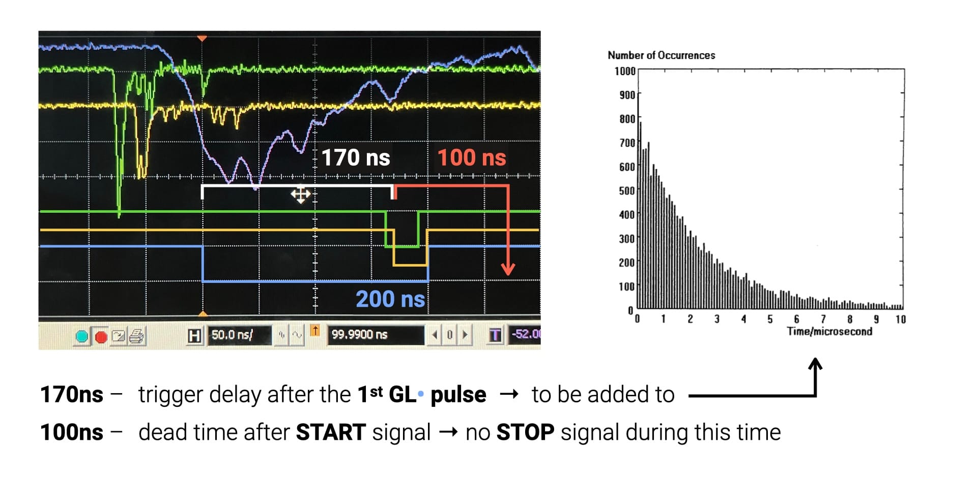
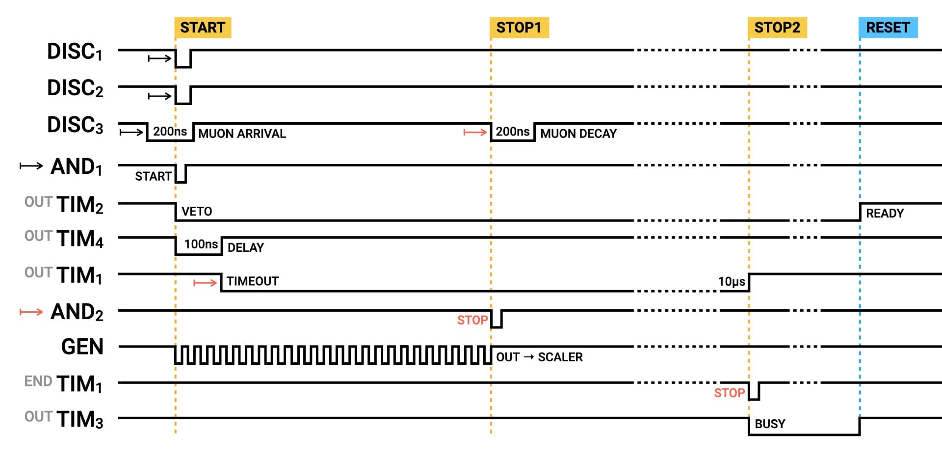
Therefore, DELAY signal in TIM4 is set to the order of 100 ns to create a dead-time window, during which we ignore any BGO pulses. The scheme below shows the timing diagram of the most important elements in this DAQ setup, including the START, RESET and the two possible STOP markers.
In this video, which I've recorded in the lab, you can see the whole setup in action, including the blinking LEDs in the NIM and CAMAC modules as well as PMT waveforms in the oscilloscope, updating after every trigger.
Measured results
After running this setup for 9 days, it has registered about 350K muons, but only about 0.6% of them actually stopped in the BGO crystal. Below you can see the time-lapse animation of the actually registered data, plotted as a histogram in the range from 1 to 10 µs.
As you can see, there is sharp increase in the number of events in the region below 2 µs, which is likely caused by very large pulses from the BGO staying above threshold even after the 100 ns DELAY. This can happen when the muon doesn't stop inside the BGO crystal, but crosses it completely. The longer scintillation path in this case creates more photons, larger current pulse in the PMT and stronger signal reflections due to impedance mismatch.
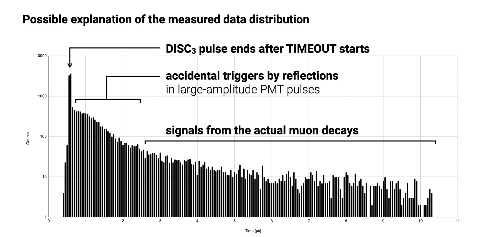
After more careful data analysis using Python, the optimal time window in this dataset was found to be from 2.5 µs to 10 µs, where the data agrees well with an exponent function with 𝜏 = 2.2 µs, while the best-fit value is obtained for 𝜏 = 2.09 ± 0.16 µs with the given statistics.
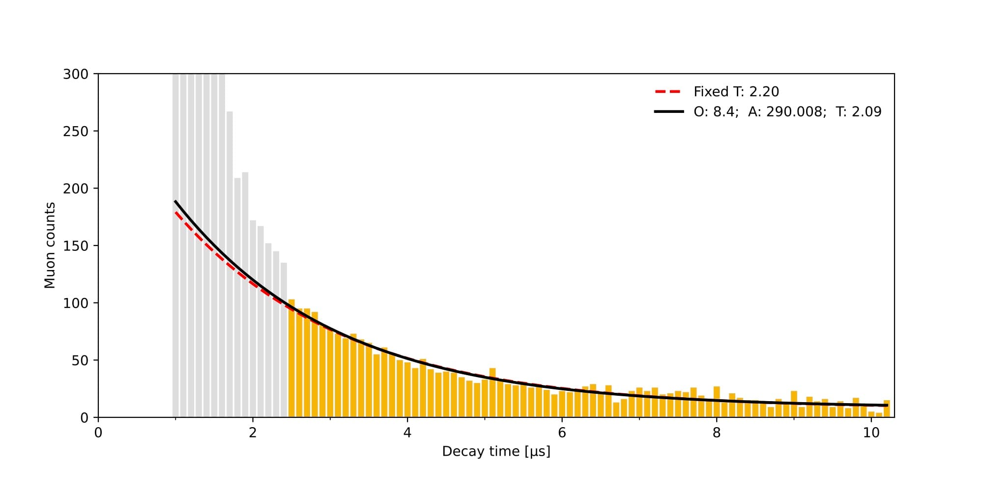
↳ f(x) = O + A • exp(-x/T)
Another aspect worth noting is the effect of muon capture by the nuclei in the BGO crystal. Negative electrons (µ-) that stopped inside the crystal can interact with protons (p) of the Bi, Ge, and O nuclei, producing a neutron (n) instead of an electron:
μ- + p → n + ν
This process can happen before the actual muon decay, which effectively reduces the measured time between the two BGO pulses. Positive muons (µ+), on the other hand, cannot participate in this process. Therefore, depending on the relative contribution of negative muons in our sample, the measured parameter 𝜏 of the exponent can be slightly lower than the actual value of the muon's mean lifetime (2.2 µs).
Improved configuration
To reduce the contribution of background signals, I've upgraded the DAQ configuration with the following 3 changes:
- the DELAY has been increased to 2 µs, which should avoid spurious STOP signals close to the 1st BGO pulse, getting a more stable baseline;
- the TIMEOUT has been increased to 100 µs, to get more bins in the tail of the exponent, which would better constrain the offset parameter (O) in the fit function;
- an ADC (Analog to Digital Converter) module has been added to the CAMAC crate to also measure the integral of the 2nd BGO pulse within a 300 ns time window around the STOP signal, which could allow to better differentiate between pulses created by an electron, a neutron or some hardware effect correlated with the 1st pulse.